Analysis of Variance

class: center, middle, inverse, title-slide

.title[
# Analysis of Variance
]
.subtitle[
## (ANOVA)
]
.author[
### Pablo E. Gutiérrez-Fonseca
]
.date[
### 2024-10-19
]

---

# What is ANOVA
- Analysis of Variance (ANOVA) is a statistical technique, commonly used to studying **differences between two or more group means**.

- ANOVA test is centered on the different sources of variation in a typical variable.

- This statistical method is an extension of the independent samples t-test for comparing the means in a situation where **there are more than two groups**.

---
# Hypothesis in one-way ANOVA test
.pull-left[
- `$H_0$`: All group means are equal.

- `$H_0: \mu_1 = \mu_2 = \mu_3 = \dots = \mu_k$`
]

.pull-right[ 
- `$H_a$`: At least, the mean of one group is different

- `$H_A: \mu_i \neq \mu_j \quad \text{for some } i, j$`
]

<center>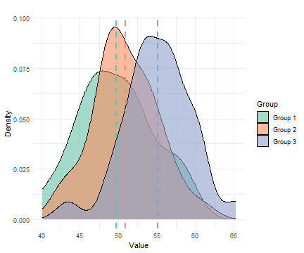
![](ANOVA_files/figure-html/unnamed-chunk-2-1.png)

---
# When would you run an ANOVA?

- I have a continuous response variable.

- I want to know the difference in that response between more than two groups.

- I have one factor I am testing (One-Way ANOVA).

---
# Decision Flowchart

<div id="htmlwidget-fbfc52d82635d988c6e1" style="width:850px;height:550px;" class="DiagrammeR html-widget "></div>
<script type="application/json" data-for="htmlwidget-fbfc52d82635d988c6e1">{"x":{"diagram":"\n graph TD;\n\n A[What type of data?] --> B[Continuous] \n A --> Z[Categorical]\n \n B --Research Question--> C[Comparing Differences] \n B --Research Question--> D[Examining Relationships]\n \n C --How many groups?--> E[1 group] \n C --How many groups?--> I[2 groups]\n C --How many groups?--> Q[> 2 groups]\n \n E --> F[Normally distributed?] \n F --Yes--> G[One sample z-test] \n F --No--> H[Wilcoxon signed rank test]\n \n I --> J[Are Samples Independent?] \n J --Yes--> K[Normally distributed?] \n J --No--> L[Normally distributed?]\n \n K --Yes--> M[Independent t-test] \n K --No--> N[Wilcoxon rank sum test] \n \n L --Yes--> O[Paired t-test] \n L --No--> P[Wilcoxon matched pair test]\n \n Q --> R[Use ANOVA] \n Q --> S[Non-parametric ANOVA]\n\n style A fill:lightblue,stroke:#333,stroke-width:1px\n style B fill:lightblue,stroke:#333,stroke-width:1px\n style C fill:lightblue,stroke:#333,stroke-width:1px\n style D fill:lightblue,stroke:#333,stroke-width:1px\n style E fill:lightblue,stroke:#333,stroke-width:1px\n style F fill:lightblue,stroke:#333,stroke-width:1px\n style G fill:lightblue,stroke:#333,stroke-width:1px\n style H fill:lightblue,stroke:#333,stroke-width:1px\n style I fill:lightblue,stroke:#333,stroke-width:1px\n style J fill:lightblue,stroke:#333,stroke-width:1px\n style K fill:lightblue,stroke:#333,stroke-width:1px\n style L fill:lightblue,stroke:#333,stroke-width:1px\n style M fill:lightblue,stroke:#333,stroke-width:1px\n style N fill:lightblue,stroke:#333,stroke-width:1px\n style O fill:lightblue,stroke:#333,stroke-width:1px\n style P fill:lightblue,stroke:#333,stroke-width:1px\n style Q fill:lightblue,stroke:#333,stroke-width:1px\n style Z fill:lightblue,stroke:#333,stroke-width:1px\n\n "},"evals":[],"jsHooks":[]}</script>

---
# Decision Flowchart: Testing Process

<div id="htmlwidget-2f4c52b7f36e26c300a7" style="width:600px;height:400px;" class="DiagrammeR html-widget "></div>
<script type="application/json" data-for="htmlwidget-2f4c52b7f36e26c300a7">{"x":{"diagram":"\n graph TD;\n\n A[Independent Samples?] --> B[Test Normality of Residuals]\n\n B --Normality Assumed--> C[Test Homogeneity of Variances]\n B --Normality Not Assumed--> F[Kruskal-Wallis Test]\n \n C --Equal Variances--> D[ANOVA]\n C --Unequal Variances--> E[Welch Test]\n\n style A fill:lightblue,stroke:#333,stroke-width:1px\n style B fill:lightblue,stroke:#333,stroke-width:1px\n style C fill:lightblue,stroke:#333,stroke-width:1px\n style D fill:lightblue,stroke:#333,stroke-width:1px\n style E fill:lightblue,stroke:#333,stroke-width:1px\n style F fill:lightblue,stroke:#333,stroke-width:1px\n "},"evals":[],"jsHooks":[]}</script>

---
# Assumptions

- All groups are Independent.

- The data is normally distributed.

- All groups have approximately equal variance.
  - A good rule of thumb: ratio of largest to smallest group stdev must be less than 2:1
  - The ANOVA is less sensitive to this requirement when samples are of equal size from each population.

---
# Assumptions

- A common misconception is that the **response variable** must be normally distributed when conducting an ANOVA. This is **incorrect** because the normality assumptions pertain to the **residuals**, not the response variable.

---
# Assumptions

- The key assumption of ANOVA is that the **residuals** **are independent** and come from a **normal distribution** with mean 0 and variance `$\sigma^2$`. Specifically:
<center>
`$y_{ij} = \mu + \alpha_i + \epsilon_{ij}$`
</center>
Where:
- `$y_{ij}$` This is the observed value of the response variable for the `$j$`-th observation in the `$i$`-th group
- `$\mu$` is the overall mean
- `$\alpha_i$` is the effect of the `$i$`-th group
- `$\epsilon_{ij} \sim \text{Normal}(0, \sigma^2)$`, where `$\epsilon_{ij}$` represents the residual error.

- Thus, it is the **residuals** `$\epsilon_{ij}$` that must be normally distributed, not the response variable `$y_{ij}$`.

---
# How ANOVA works 
- The ANOVA obtained value (the **F-statistic**) is a ratio of the Between Group Variation divided by the Within Group Variation:

<center>
F = `$\frac{\text{Between-group variance}}{\text{Within-group variance}}$`

- A large **F** is evidence against `$H_0$`, since it indicates that there is more difference between groups than within groups.

---
# Finding the critical value for an F-test

.pull-left[ 
- You will need the critical F table that matches your significance level.

- And you will need to know the degrees of freedom for both the between and within variability.

]

.pull-right[ 
<img src="fig/f-table.png" alt="Degrees of Freedom T-Table" width="600"/>
]

---

# One-way ANOVA Summary Table

| Source of Variation | Degrees of Freedom (DF) | Sum of Squares (SS) | Mean Square (MS) | F-value |
|----------------------------------|:----------------------------------:|:----------------------------------:|:---------------------------:|:---------------------:|
| **Between Groups** | `$c - 1$` | `$SSB$` | `$MSB = \frac{SSB}{c - 1}$` | `$\frac{MSB}{MSW}$` |
| **Within Groups** | `$n - c$` | `$SSW$` | `$MSW = \frac{SSW}{n - c}$` | |
| **Total** | `$n - 1$` | `$SST = SSB + SSW$` | | |

- `$c$` = number of groups.  
- `$n$` = number of observations.

---
# One-way ANOVA Formulas

.pull-left[ 
- The formula for the Sum of Squares Between (SSB) is given by:
$$ SSB = \sum_{j=1}^{C} n_j (\bar{x}_j - \bar{x})^2 $$

Where:
- `$C$` = number of groups
- `$n_j$` = sample size of group `$j$`
- `$\bar{x}_j$` = mean of group `$j$`
- `$\bar{x}$` = overall mean
]

.pull-right[ ]

---
# One-way ANOVA Formulas

.pull-left[ 
- The formula for the Sum of Squares Between (SSB) is given by:
$$ SSB = \sum_{j=1}^{C} n_j (\bar{x}_j - \bar{x})^2 $$

Where:
- `$C$` = number of groups
- `$n_j$` = sample size of group `$j$`
- `$\bar{x}_j$` = mean of group `$j$`
- `$\bar{x}$` = overall mean
]

.pull-right[
- The formula for the Sum of Squares Within (SSW) is given by:

`$$SSW = \sum_{j=1}^{C} \sum_{i=1}^{n_j} (\bar{x}_j - \bar{x})^2$$`

Where:
- `$C$` = number of groups
- `$n_j$` = sample size of group `$j$`
- `$\bar{x}_j$` = mean of group `$j$`
- `$\bar{x}$` = overall mean
]

---
# One-way ANOVA Summary Table
- In a study on plant growth with a sample size of **40**, **six different fertilizer** types were tested.

---
# One-way ANOVA Summary Table
- In a study on plant growth with a sample size of **40**, **six different fertilizer** types were tested..

| Source of Variation | Degrees of Freedom (DF) | Sum of Squares (SS) | Mean Square (MS) | F-value |
|----------------------------------|:----------------------------------:|:----------------------------------:|:---------------------------:|:---------------------:|
| **Between Groups** | `$c - 1$` | 2150 | `$MSB = \frac{SSB}{c - 1}$` | `$\frac{MSB}{MSW}$` |
| **Within Groups** | `$n - c$` | 5269 | `$MSW = \frac{SSW}{n - c}$` | |
| **Total** | `$n - 1$` | `$SST = SSB + SSW$` | | |

- `$c$` = number of groups.  
- `$n$` = number of observations.

---
# One-way ANOVA Summary Table
- In a study on plant growth with a sample size of **40**, **six different fertilizer** types were tested..

| Source of Variation | Degrees of Freedom (DF) | Sum of Squares (SS) | Mean Square (MS) | F-value |
|----------------------------------|:----------------------------------:|:----------------------------------:|:---------------------------:|:---------------------:|
| **Between Groups** | 5 | 2150 | `$MSB = \frac{SSB}{c - 1}$` | `$\frac{MSB}{MSW}$` |
| **Within Groups** | `$n - c$` | 5269 | `$MSW = \frac{SSW}{n - c}$` | |
| **Total** | `$n - 1$` | `$SST = SSB + SSW$` | | |

- `$c$` = number of groups.  
- `$n$` = number of observations.

---
# One-way ANOVA Summary Table
- In a study on plant growth with a sample size of **40**, **six different fertilizer** types were tested..

| Source of Variation | Degrees of Freedom (DF) | Sum of Squares (SS) | Mean Square (MS) | F-value |
|----------------------------------|:----------------------------------:|:----------------------------------:|:---------------------------:|:---------------------:|
| **Between Groups** | 5 | 2150 | `$MSB = \frac{SSB}{c - 1}$` | `$\frac{MSB}{MSW}$` |
| **Within Groups** | 34 | 5269 | `$MSW = \frac{SSW}{n - c}$` | |
| **Total** | `$n - 1$` | `$SST = SSB + SSW$` | | |

- `$c$` = number of groups.  
- `$n$` = number of observations.

---
# One-way ANOVA Summary Table
- In a study on plant growth with a sample size of **40**, **six different fertilizer** types were tested..

| Source of Variation | Degrees of Freedom (DF) | Sum of Squares (SS) | Mean Square (MS) | F-value |
|----------------------------------|:----------------------------------:|:----------------------------------:|:---------------------------:|:---------------------:|
| **Between Groups** | 5 | 2150 | `$MSB = \frac{SSB}{c - 1}$` | `$\frac{MSB}{MSW}$` |
| **Within Groups** | 34 | 5269 | `$MSW = \frac{SSW}{n - c}$` | |
| **Total** | 39 | `$SST = SSB + SSW$` | | |

- `$c$` = number of groups.  
- `$n$` = number of observations.

---
# One-way ANOVA Summary Table
- In a study on plant growth with a sample size of **40**, **six different fertilizer** types were tested.

| Source of Variation | Degrees of Freedom (DF) | Sum of Squares (SS) | Mean Square (MS) | F-value |
|----------------------------------|:----------------------------------:|:----------------------------------:|:---------------------------:|:---------------------:|
| **Between Groups** | 5 | 2150 | `$MSB = \frac{SSB}{c - 1}$` | `$\frac{MSB}{MSW}$` |
| **Within Groups** | 34 | 5269 | `$MSW = \frac{SSW}{n - c}$` | |
| **Total** | 39 | 7419 | | |

- `$c$` = number of groups.  
- `$n$` = number of observations.

---
# One-way ANOVA Summary Table
- In a study on plant growth with a sample size of **40**, **six different fertilizer** types were tested.

| Source of Variation | Degrees of Freedom (DF) | Sum of Squares (SS) | Mean Square (MS) | F-value |
|----------------------------------|:----------------------------------:|:----------------------------------:|:---------------------------:|:---------------------:|
| **Between Groups** | 5 | 2150 | 430 | `$\frac{MSB}{MSW}$` |
| **Within Groups** | 34 | 5269 | `$MSW = \frac{SSW}{n - c}$` | |
| **Total** | 39 | 7419 | | |

- `$c$` = number of groups.  
- `$n$` = number of observations.

---
# One-way ANOVA Summary Table
- In a study on plant growth with a sample size of **40**, **six different fertilizer** types were tested.

| Source of Variation | Degrees of Freedom (DF) | Sum of Squares (SS) | Mean Square (MS) | F-value |
|----------------------------------|:----------------------------------:|:----------------------------------:|:---------------------------:|:---------------------:|
| **Between Groups** | 5 | 2150 | 430 | `$\frac{MSB}{MSW}$` |
| **Within Groups** | 34 | 5269 | 155 | |
| **Total** | 39 | 7419 | | |

- `$c$` = number of groups.  
- `$n$` = number of observations.

---
# One-way ANOVA Summary Table
- In a study on plant growth with a sample size of **40**, **six different fertilizer** types were tested.

| Source of Variation | Degrees of Freedom (DF) | Sum of Squares (SS) | Mean Square (MS) | F-value |
|----------------------------------|:----------------------------------:|:----------------------------------:|:---------------------------:|:---------------------:|
| **Between Groups** | 5 | 2150 | 430 | 2.77 |
| **Within Groups** | 34 | 5269 | 155 | |
| **Total** | 39 | 7419 | | |

- `$c$` = number of groups.  
- `$n$` = number of observations.

---
# One-way ANOVA Summary Table
- In a study on plant growth with a sample size of **40**, **six different fertilizer** types were tested.

| Source of Variation | Degrees of Freedom (DF) | Sum of Squares (SS) | Mean Square (MS) | F-value |
|----------------------------------|:----------------------------------:|:----------------------------------:|:---------------------------:|:---------------------:|
| **Between Groups** | 5 | 2150 | 430 | 2.77 |
| **Within Groups** | 34 | 5269 | 155 | |
| **Total** | 39 | 7419 | | |

- `$c$` = number of groups. 
- `$n$` = number of observations.
- `p_value <- 1 - pf(f_statistic, df_B, df_W)` = **0.03326991**

---
# Effect Size Measures
- Significant **F ratios** indicate that there is a difference between the treatment groups that cannot be explained by chance alone.
  
- Effect size measures help determine how big or meaningful the effect of the treatment is.

---
# Effect Size Measures
- One simple effect size measure:
<center>
`$r^2 = \frac{\text{SSB}}{\text{SST}}$`

Where:
  - **SSB** is the sum of squares between groups (variability due to group differences),
  - **SST** is the total sum of squares (total variability in the dataset).

- This measure shows how much of the total variability in the data can be explained by the different groupings.   
- **What is meaningful?**  
It depends on how much of the total variability you would expect this grouping to account for.

---
# One-way ANOVA Summary Table
- In a study on plant growth with a sample size of **40**, **six different fertilizer** types were tested.

| Source of Variation | Degrees of Freedom (DF) | Sum of Squares (SS) | Mean Square (MS) | F-value |
|----------------------------------|:----------------------------------:|:----------------------------------:|:---------------------------:|:---------------------:|
| **Between Groups** | 5 | 2150 | 430 | 2.77 |
| **Within Groups** | 34 | 5269 | 155 | |
| **Total** | 39 | 7419 | | |

- `$c$` = number of groups. 
- `$n$` = number of observations.
- `p_value <- 1 - pf(f_statistic, df_B, df_W)` = **0.03326991**
- `$r^2 = \frac{SSB}{SST} = \frac{2150}{7419}$` = **0.2897**

---
# Example

``` r
crop <- read.csv('Lecturer Practice/crop.csv')
head(crop)
```

```
##   density block fertilizer    yield
## 1       1     1       ctrl 177.2287
## 2       2     2       ctrl 177.5500
## 3       1     3       ctrl 176.4085
## 4       2     4       ctrl 177.7036
## 5       1     1       ctrl 177.1255
## 6       2     2       ctrl 176.7783
```

---
# Data visualization
- Visualize the data distribution using boxplots and jitter for individual points:

.panelset[
.panel[.panel-name[R Code]

``` r
ggplot(crop) +
  aes(x = fertilizer, y = yield, fill = fertilizer) +
  geom_boxplot() +
    geom_jitter(shape = 15,
        color = "steelblue",
        position = position_jitter(0.21)) +
   theme_minimal()
```
]

.panel[.panel-name[Plot]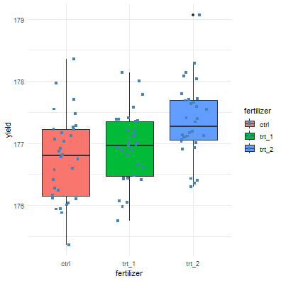
![](ANOVA_files/figure-html/plot1-1.png)
]
]

---
# Running the ANOVA
- Run one-way ANOVA to assess differences between fertilizer groups:

``` r
one.way <- aov(yield ~ fertilizer, 
 data = crop, var.equal = TRUE )

summary(one.way)
```

```
##             Df Sum Sq Mean Sq F value Pr(>F)    
*## fertilizer   2   6.07  3.0340   7.863 0.0007 ***
## Residuals   93  35.89  0.3859                   
## ---
## Signif. codes:  0 '***' 0.001 '**' 0.01 '*' 0.05 '.' 0.1 ' ' 1
```

---
# Checking Assumptions

---
# Checking Assumptions
- ANOVA assumes that **residuals** are **normally distributed** and that the **variance across groups is homogeneous (equal variances)**.

- The **normality of residuals** can be tested using the **Shapiro-Wilk test**.

- The **homogeneity of variances** can be checked using **Bartlett's test** or **Levene's test**.

- Additionally, diagnostic plots like **Q-Q plots (for normality)** and **Residuals vs. Fitted plots (for homogeneity)** can provide visual confirmation.

---
# Checking Assumptions: Normality
- Check normality of residuals using a QQ plot and the Shapiro-Wilk test.

.pull-left[

``` r
plot(one.way, 2)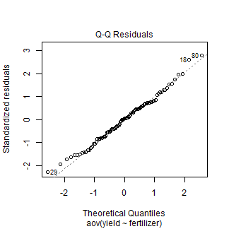 
```

![](ANOVA_files/figure-html/unnamed-chunk-6-1.png)
]

.pull-right[
]

---
# Checking Assumptions: Normality
- Check normality of residuals using a QQ plot and the Shapiro-Wilk test.

.pull-left[

``` r
plot(one.way, 2) 
```

![](ANOVA_files/figure-html/unnamed-chunk-7-1.png)
]

.pull-right[
- Compute Shapiro-Wilk test of normality

``` r
shapiro.test(residuals(one.way))
```

```
## 
## 	Shapiro-Wilk normality test
## 
## data:  residuals(one.way)
*## W = 0.99088, p-value = 0.7594
```
]

---
# Assumption Check: Interpretation 
- **QQ plot:** As the points fall approximately along the reference line, we **assume normality**.

- **Shapiro-Wilk test:** The p-value (p = 0.7594) is not significant, supporting the **assumption of normality**.

---
# Check Assumptions: Homogeneity of Variances

---
# Check Assumptions: Homogeneity of Variances
- The Residuals vs. Fits plot helps check for homogeneity of variances.

.pull-left[

``` r
plot(one.way, 1)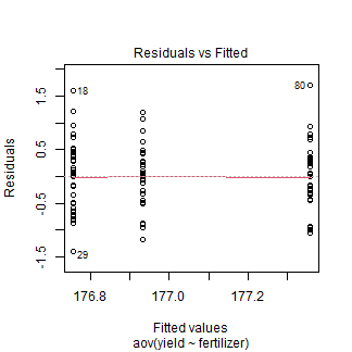 
```

![](ANOVA_files/figure-html/unnamed-chunk-9-1.png)
]

.pull-right[
In the plot above, there's no clear pattern between residuals and fitted values (the group means), which indicates **homogeneity of variances**.
]

---
# Check Assumptions: Homogeneity of Variances
.pull-left[
The homogeneity of variances can also be checked using **Bartlett's** or Levene's tests.
]

.pull-right[

``` r
bartlett.test(yield ~ fertilizer, data=crop)
```

```
## 
## 	Bartlett test of homogeneity of variances
## 
## data:  yield by fertilizer
*## Bartlett's K-squared = 1.0622, df = 2, p-value = 0.5879
```

]

---
# Check Assumptions: Homogeneity of Variances
.pull-left[
The homogeneity of variances can also be checked using Bartlett's or **Levene's tests**.
]

.pull-right[

``` r
leveneTest(yield ~ fertilizer, data=crop)
```

```
## Levene's Test for Homogeneity of Variance (center = median)
##       Df F value Pr(>F)
*## group  2  0.8472 0.4319
##       93
```

]

---
# Assumption Check: Interpretation 
- The p-value is not less than the significance level of 0.05, as seen in the output above. This indicates that **there is no indication that the variance across groups is statistically significant**.

- As a result, we can infer that the **variations in the different treatment groups are homogeneous**.

---
# Post-hoc test

## Why Perform a Post-hoc Test?

- When the **overall p-value** from the ANOVA is below the significance level (typically p < 0.05), it suggests that **at least one group mean is different from the others**.

- However, ANOVA does not specify which groups are different; it only tells us that **not all group means are equal**.

- To pinpoint which groups differ, we need to conduct a **post-hoc test**. This test controls for the family-wise error rate, ensuring accurate comparisons between group means.

---
# Post-hoc test

## Why Perform a Post-hoc Test?

- Two of the most commonly used post-hoc tests include:

.pull-left[
- **The Tukey Method:**  
The Tukey post-hoc test should be used when you would like to make pairwise comparisons between group means when the sample sizes for each group are equal.]
.pull-right[
- **The Bonferroni Method:**  
The Bonferroni post-hoc test should be used when you have a set of planned comparisons you would like to make beforehand.
]

---
# Post-hoc test

- Since there are 3 groups (fertilizers), we will make these pairwise comparisons:

- Group 1 vs. Group 2
  - Group 1 vs. Group 3
  - Group 2 vs. Group 3
  
---
# Running the Post-hoc Test

- We use the Tukey Honest Significant Difference (Tukey HSD) test to compare all possible pairs of groups:

``` r
post_test <- TukeyHSD(one.way)
post_test 
```

```
##   Tukey multiple comparisons of means
##     95% family-wise confidence level
## 
## Fit: aov(formula = yield ~ fertilizer, data = crop, var.equal = TRUE)
## 
## $fertilizer
##                  diff         lwr       upr     p adj
*## trt_1-ctrl  0.1761687 -0.19371896 0.5460564 0.4954705
*## trt_2-ctrl  0.5991256  0.22923789 0.9690133 0.0006125
*## trt_2-trt_1 0.4229568  0.05306916 0.7928445 0.0208735
```

---
# Visualizing the Post-hoc Test

- The plot below visualizes the results of the Tukey HSD test:

``` r
plot(post_test)
```

![](ANOVA_files/figure-html/unnamed-chunk-13-1.png)

---
# How to summarize results

- State the original research question / hypothesis. 
- Briefly describe the methods including the type of test run: One-way ANOVA, if significant type of Means Comparison (e.g. Tukey's HSD Means Comparison). 
- Describe your results including: Shorthand: `$F_{(df_1, df_2)} = , p-value , r^2 =$`. Results of any means comparison (which groups are larger than which other groups? Which are the same?). 
- Interpret significance and effect size ( `$r^2$` ), big picture: what does this mean in terms of your original research question?