class: center, middle, inverse, title-slide .title[ # Correlations and Partial Correlations in R ] .author[ ### Pablo E. Gutiérrez-Fonseca ] .date[ ### 2024-11-04 ] --- # Decision Flowchart <div id="htmlwidget-389d51e62a13c4ce9bf0" style="width:1000px;height:500px;" class="DiagrammeR html-widget "></div> <script type="application/json" data-for="htmlwidget-389d51e62a13c4ce9bf0">{"x":{"diagram":"\n graph TD;\n\n A[What type of data?] --> B[Continuous] \n A --> C[Categorical]\n \n B --Research Question--> D[Comparing Differences] \n B --Research Question--> E[Examining Relationships]\n \n D --> F[How many groups?] \n \n F --1 group--> G[Normally distributed?] \n G --Yes--> H[One-sample z-test] \n G --No--> I[Wilcoxon signed rank test]\n \n F --2 groups--> J[Are Samples Independent?] \n J --Yes--> K[Normally distributed?]\n J --No--> L[Normally distributed?]\n \n K --Yes--> M[Independent t-test] \n K --No--> N[Wilcoxon rank sum test] \n \n L --Yes--> O[Paired t-test] \n L --No--> P[Wilcoxon matched pair test]\n \n F --More than 2 groups--> Q[Number of Treatments?]\n \n Q --One--> R[Normally Distributed?]\n R --Yes--> S[One-Way ANOVA]\n R --No--> T[Non-Parametric ANOVA]\n \n Q --More than One--> U[Normally Distributed?]\n \n U --Yes--> V[Factorial ANOVA]\n U --No--> W[Friedman's Rank Test]\n \n E --> X[Number of Treatment Variables?]\n \n X --Two--> Y[Normally Distributed?]\n Y --Yes--> Z[Pearson's Correlation]\n Y --No--> AA[Spearman's Rho]\n \n X --More than Two--> AB[Partial Correlation]\n\n style A fill:lightblue,stroke:#333,stroke-width:1px, fontSize: 18px\n style B fill:lightblue,stroke:#333,stroke-width:1px, fontSize: 18px\n style C fill:lightblue,stroke:#333,stroke-width:1px, fontSize: 18px\n style D fill:lightblue,stroke:#333,stroke-width:1px, fontSize: 18px\n style E fill:lightblue,stroke:#333,stroke-width:1px, fontSize: 18px\n style F fill:lightblue,stroke:#333,stroke-width:1px, fontSize: 18px\n style G fill:lightblue,stroke:#333,stroke-width:1px, fontSize: 18px\n style H fill:lightblue,stroke:#333,stroke-width:1px, fontSize: 18px\n style I fill:lightblue,stroke:#333,stroke-width:1px, fontSize: 18px\n style J fill:lightblue,stroke:#333,stroke-width:1px, fontSize: 18px\n style K fill:lightblue,stroke:#333,stroke-width:1px, fontSize: 18px\n style L fill:lightblue,stroke:#333,stroke-width:1px, fontSize: 18px\n style M fill:lightblue,stroke:#333,stroke-width:1px, fontSize: 18px\n style N fill:lightblue,stroke:#333,stroke-width:1px, fontSize: 18px\n style O fill:lightblue,stroke:#333,stroke-width:1px, fontSize: 18px\n style P fill:lightblue,stroke:#333,stroke-width:1px, fontSize: 18px\n style Q fill:lightblue,stroke:#333,stroke-width:1px, fontSize: 18px\n style R fill:lightblue,stroke:#333,stroke-width:1px, fontSize: 18px\n style S fill:lightblue,stroke:#333,stroke-width:1px, fontSize: 18px\n style T fill:lightblue,stroke:#333,stroke-width:1px, fontSize: 18px\n style U fill:lightblue,stroke:#333,stroke-width:1px, fontSize: 18px\n style V fill:lightblue,stroke:#333,stroke-width:1px, fontSize: 18px\n style W fill:lightblue,stroke:#333,stroke-width:1px, fontSize: 18px\n style X fill:lightblue,stroke:#333,stroke-width:1px, fontSize: 18px\n style Y fill:lightblue,stroke:#333,stroke-width:1px, fontSize: 18px\n style Z fill:lightblue,stroke:#333,stroke-width:1px, fontSize: 18px\n style AA fill:lightblue,stroke:#333,stroke-width:1px, fontSize: 18px\n style AB fill:lightblue,stroke:#333,stroke-width:1px, fontSize: 18px\n\n "},"evals":[],"jsHooks":[]}</script> --- # What is Correlation? - A correlation test quantifies how two variables change together. - Are the variables closely related? - To what extent does one variable predict the other? --- # When to Use Correlation? - Correlation test is used to **evaluate** the **association between two or more variables**. - You have two continuous variables measured from the same observational unit. - You want to determine if the variables are related (vary in unison). --- # Key Assumptions: - Independent, random samples. - Normality: - Pearson correlation (parametric): Assumes both variables follow a normal distribution. - Spearman correlation (nonparametric): Does not assume normality. - Linear relationship: Correlation looks for a linear association between the variables. --- # Describing Correlations - **Strength**: Indicates how closely the variables are related. - Categories: Weak, Moderate, Strong - **Nature**: Shows the direction of the relationship. - Direct (Positive): As one variable increases, so does the other. - Indirect (Negative): As one variable increases, the other decreases. - **Significance**: Assesses if the correlation is meaningful. - Based on the p-value, which tells us if the observed relationship is likely due to chance. --- # Hypothesis testing with Correlations - Null Hypothesis ( `\(H_0\)` ) - ** `\(H_0\)` **: There is no correlation in the population. - For a two-tailed test, this means there is **no linear relationship** between x and y. $$ H_0: r = 0 $$ $$ p > 0.05 $$ - Alternative Hypothesis ( `\(H_1\)` ) - ** `\(H_1\)` **: There is a real, non-zero correlation in the population. - The alternative hypothesis suggests a **significant linear relationship** between x and y. $$ H_1: r \neq 0 $$ $$ p < 0.05 $$ --- # Computing Simple Correlations - There are many kinds of correlation coefficients but the most commonly used measure of correlation is the **Pearson’s correlation (parametric statistic)**. `$$r_{XY} = \frac{n \sum XY - \left( \sum X \right) \left( \sum Y \right)}{\sqrt{\left[ n \sum X^2 - \left( \sum X \right)^2 \right] \left[ n \sum Y^2 - \left( \sum Y \right)^2 \right]}}$$` --- # Computing Simple Correlations - There are many kinds of correlation coefficients but the most commonly used measure of correlation is the **Pearson’s correlation (parametric statistic)**. `$$r_{XY} = \frac{n \sum XY - \left( \sum X \right) \left( \sum Y \right)}{\sqrt{\left[ n \sum X^2 - \left( \sum X \right)^2 \right] \left[ n \sum Y^2 - \left( \sum Y \right)^2 \right]}}$$` Where: - `\(r\)` = Pearson Correlation Coefficient - `\(N\)` = Number of pairs of observations - `\(∑XY\)` = Sum of the products of paired values - `\(∑X\)` = Sum of the \(x\) scores - `\(∑Y\)` = Sum of the \(y\) scores - `\(∑X^2\)` = Sum of the squared \(x\) scores - `\(∑Y^2\)` = Sum of the squared \(y\) scores --- # Nature and Interpretation of `\(r\)` Value .pull-left[ - Perfect **Positive Correlation**: `\(r=+1\)` - All points lie on an upward-sloping line. ] .pull-right[ 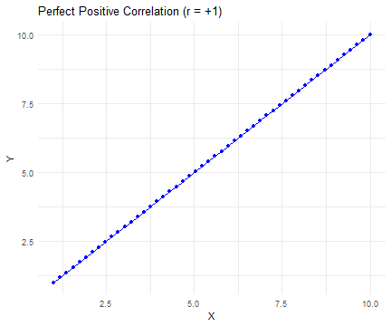<!-- --> ] --- # Nature and Interpretation of `\(r\)` Value .pull-left[ - Perfect Positive Correlation: `\(r=+1\)` - All points lie on an upward-sloping line. - **No Correlation**: `\(r=0\)` - Points do not align along any line, or they form a horizontal line. ] .pull-right[ 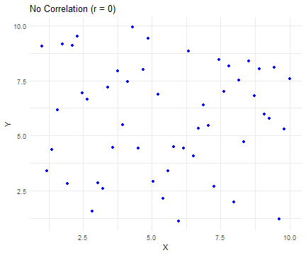<!-- --> ] --- # Nature and Interpretation of `\(r\)` Value .pull-left[ - Perfect Positive Correlation: `\(r=+1\)` - All points lie on an upward-sloping line. - No Correlation: `\(r=0\)` - Points do not align along any line, or they form a horizontal line. - Perfect **Negative Correlation**: `\(r=−1\)` - All points lie on a downward-sloping line. ] .pull-right[ 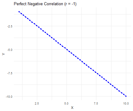<!-- --> ] --- # Nature and Interpretation of `\(r\)` Value .pull-left[ - Perfect **Positive Correlation**: `\(r=+1\)` - All points lie on an upward-sloping line. - No Correlation: `\(r=0\)` - Points do not align along any line, or they form a horizontal line. - Perfect **Negative Correlation**: `\(r=−1\)` - All points lie on a downward-sloping line. ] .pull-right[ <!-- --> ] - Note: When `\(∣r∣=1\)`, we have a perfect correlation, meaning all points fall precisely along a straight line. --- # Strength of Correlation .pull-left[ - Weak Correlation: - `\(0.0≤ ∣r∣ <0.3\)` - Moderate Correlation: - `\(0.3≤∣r∣<0.7\)` - Strong Correlation: - `\(0.7≤∣r∣<1.0\)` - Perfect Correlation: - `\(∣r∣=1.0\)` ] .pull-right[ 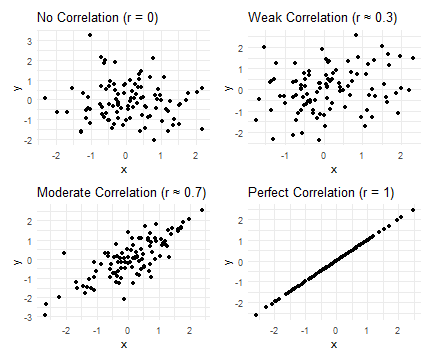<!-- --> ] --- # Strength of Correlation: Examples .pull-left[ - Weak Correlation: - `\(0.0≤ ∣r∣ <0.3\)` - Moderate Correlation: - `\(0.3≤∣r∣<0.7\)` - Strong Correlation: - `\(0.7≤∣r∣<1.0\)` - Perfect Correlation: - `\(∣r∣=1.0\)` ] .pull-right[ - Husband’s age / Wife’s age: - r = .94 (strong positive correlation) - Husband’s height / Wife’s height: - r = .36 (weak positive correlation) - Distance of golf putt / percent success: - r = -.94 (strong negative correlation) ] --- # Coefficient of Determination ( `\(r^2\)` ) - `\(r^2\)` quantifies the proportion of variability in one variable that can be explained by its relationship with the other variable. - It represents the shared variability between the two variables, indicating how much of the total variability they have in common. - When two variables are correlated, `\(r^2\)` tells us how much variance in one variable can be accounted for by the other. - This concept is similar to the Effect Size we examined in ANOVA. --- # Difference between `\(r\)` and `\(r^2\)` - `\(r\)` (Pearson’s Correlation Coefficient): - Measures how much two variables vary together. - Ranges from -1 to 1: - -1: Perfect negative correlation - 0: No correlation - 1: Perfect positive correlation - Unitless and applicable across contexts. --- # Difference between `\(r\)` and `\(r^2\)` - `\(r\)` (Pearson’s Correlation Coefficient): - Measures how much two variables vary together. - Ranges from -1 to 1: - -1: Perfect negative correlation - 0: No correlation - 1: Perfect positive correlation - Unitless and applicable across contexts. - `\(r^2\)` (Coefficient of Determination): - Indicates the proportion of variability explained by the relationship. - Ranges from 0 to 1: - 0: No variability explained - 1: All variability explained - Interpreted as the percentage of variance explained. --- # p-value of the correlation The p-value (significance level) of the correlation can be determined : - by using the correlation coefficient table for the degrees of freedom : **df= n−2**, where **n is the number of observation in x and y variables**. --- # p-value of the correlation The p-value (significance level) of the correlation can be determined : - by using the correlation coefficient table for the degrees of freedom : **df= n−2**, where **n is the number of observation in x and y variables**. - or by calculating the t value as follow: $$ t = \frac{r_1 - r_2}{\sqrt{\frac{1 - r^2}{n - 2}}} $$ In the case 2) the corresponding p-value is determined using t distribution table for df=n−2 --- # Understanding significant correlations - **Significant correlations** indicate that fluctuations in the values are sufficiently regular, making it unlikely that the association occurred by chance. - However, significance does not imply meaningfulness: - A significant correlation does not guarantee that the amount of variance accounted for is practically significant. - Use ** `\(r^2\)` to assess the meaningfulness** of your results: - Interpret `\(r^2\)` to understand the proportion of variance explained by the correlation and its practical implications. --- # Writing Up Your Results .pull-left[ Example: - Correlation Results: `\(r_{(19)}=0.606, p=0.024, r^2=0.37\)` ] --- # Writing Up Your Results .pull-left[ Example: - Correlation Results: `\(r_{(19)}=0.606, p=0.024, r^2=0.37\)` Interpretation: - r: - Test Statistic: 0.606 (obtained value) - Indicates a moderate positive correlation between the variables. Degrees of Freedom: - 19 (calculated as `\(n−2\)`, where `\(n\)` is the number of observations). ] .pull-right[ p-value: - 0.024: Indicates a statistically significant correlation (p < 0.05), suggesting the correlation is unlikely to have arisen by chance. `\(r^2\)`: - 0.37: Indicates that approximately 37% of the variance in one variable is explained by the other, providing a measure of the correlation's practical significance. ] --- # Complications and limitations of correlation --- # Complications and limitations of correlation .pull-left[ - Sensitivity to Outliers: - Correlations can be significantly affected by outliers, which may skew the results. - Influence of Outliers: - A single outlier can have a disproportionate impact on the correlation coefficient, potentially leading to misleading conclusions. ] .pull-right[ <!-- --> ] --- # Complications and limitations of correlation - **Spurious Correlations**: - A significant correlation may not indicate a direct relationship between the two variables. - It can arise from an indirect correlation influenced by a third variable. - For example, an observed correlation between ice cream sales and drowning incidents might be spurious, driven by a third factor like temperature. - **Causation vs. Correlation**: - Correlation does not imply causation. Just because two variables are correlated does not mean one causes the other. - **Context Matters**: - Always consider the context and underlying mechanisms that could affect the relationship between the variables. --- # Multivariate interpretation - What to Do? --- # Multivariate interpretation - What to Do? - Check out your Partial Correlations. - Purpose: These correlations adjust each correlation to account for the influence of all other variables in the analysis. - Benefit: They reveal the unique relationship between variables by removing the influence of others. - When to use: Conduct this analysis only on variables that significantly correlate with your variable of interest. --- # Partial Correlations - Keep in Mind: - These new partial correlations have been adjusted for covariance with all other variables. - The goal is to isolate the unique covariance between the two variables of interest. - Important Note: - Expect these values to be lower than the original correlations! - Why? Because we are accounting for the influence of other variables. - Focus on relative strength rather than trying to meet an absolute threshold of strength. --- # Other complications - Quantifying Relationships: Pearson’s, Spearman’s non-parametric, and Partial Correlations are all designed to quantify linear relationships. - They will not detect nonlinear relationships. - Misleading Data: Correlations using rates and averages (smoothed data) can be misleading. --- # Things to remember - Correlations only tell us about the strength of a linear relationship between two variables. - We cannot interpret causality from correlation alone. --- # Spearman correlation formula The Spearman correlation method computes the correlation between the rank of `\(x\)` and the rank of `\(y\)` variables: `$$\rho = \frac{\sum (x' - \bar{X}) (y' - \bar{Y})}{\sqrt{\sum (x' - \bar{X})^2 \sum (y' - \bar{Y})^2}}$$` Where `\(x' = rank(x)\)` and `\(y' = rank(y)\)`. --- # Example --- # Examining the relationship between CO₂ and Global Temperature **Load Data**: Import the dataset containing global temperature and CO₂ concentration. ``` r global_T <- read_xlsx('Lecturer Practice/global mean T.xlsx') tail(global_T) ``` ``` ## # A tibble: 6 × 3 ## year temperature Mona_Loa_co2 ## <dbl> <dbl> <dbl> ## 1 2013 14.6 397. ## 2 2014 14.7 399. ## 3 2015 14.8 401. ## 4 2016 14.9 404. ## 5 2017 14.8 407. ## 6 2018 14.7 409. ``` --- # Relationship between CO₂ and Temperature **Test for Normality**: Use Shapiro-Wilk tests to check if temperature and Mona_Loa_co2 are normally distributed. ``` r shapiro.test(global_T$temperature) ``` ``` ## ## Shapiro-Wilk normality test ## ## data: global_T$temperature *## W = 0.9314, p-value = 0.000002771 ``` --- # Relationship between CO₂ and Temperature **Test for Normality**: Use Shapiro-Wilk tests to check if temperature and Mona_Loa_co2 are normally distributed. ``` r shapiro.test(global_T$Mona_Loa_co2) ``` ``` ## ## Shapiro-Wilk normality test ## ## data: global_T$Mona_Loa_co2 *## W = 0.94085, p-value = 0.005914 ``` --- # Relationship between CO₂ and Temperature This code performs a **Spearman correlation** test to examine the relationship between global temperature and CO₂ concentration. ``` r #Test correlation (parametric) test <- cor.test(global_T$temperature, global_T$Mona_Loa_co2, method = "spearman") test ``` ``` ## ## Spearman's rank correlation rho ## ## data: global_T$temperature and global_T$Mona_Loa_co2 *## S = 2403.6, p-value < 0.00000000000000022 ## alternative hypothesis: true rho is not equal to 0 ## sample estimates: ## rho *## 0.9332148 ``` --- # Coefficient of Determination (R²) for Spearman Correlation Approximate the proportion of variance in temperature explained by CO₂ concentration. ``` r rho <- test$estimate # Spearman correlation coefficient R_squared <- rho^2 R_squared ``` ``` ## rho ## 0.8708898 ``` ``` r # Extract correlation coefficient and p-value p_value <- test$p.value ``` --- # Data visualization .panelset[ .panel[.panel-name[R Code] ``` r ggplot(global_T, aes(x = Mona_Loa_co2, y = temperature)) + geom_line() + geom_point() + geom_smooth() + # ylim(14,14.75) + labs(x = "CO2 (ppm)", y = "Temperature (C)", title = "") + annotate("text", x = 350, y = 14.8, label = paste("Spearman's correlation =", round(rho, 2), "\n", "p =", format.pval(p_value)), hjust = 1, vjust = 0) ``` ] .panel[.panel-name[Plot]  ] ] --- # How to summarize results <span style="color:#00796B;">We set out to examine the relationship between CO2 concentrations and global mean temperatures based on 60 years of observations at the Mona Loa Observatory. </span> <span style="color:#E65100;"> A Spearman’s rho correlation</span><span style="color:#1E88E5;"> identified an extremely strong, significant direct correlation ( `\(rho_{(58)} =0.93, p<0.001 , r^2 =0.87\)` ) </span><span style="color:#424242;"> This indicates that of all the myriad of factors that influence global mean temperatures, the concentration of ONE gas alone can account for 87% of the variability witnessed over the past six decades. This information strongly suggests that CO2 emissions have contributed to warming trends witnessed over the past half century.</span> --- # Example --- # Example: Partial Correlation Analysis --- # Partial Correlation Analysis - Explore the relationships between variables in the dataset while controlling for the influence of other variables. ``` r df <- data.frame( x= c(1,2,3,4,5,6,7,7,7,8), y= c(4,5,6,7,8,9,9,9,10,10), z= c(1,3,5,7,9,11,13,15,17,19)) head(df) ``` ``` ## x y z ## 1 1 4 1 ## 2 2 5 3 ## 3 3 6 5 ## 4 4 7 7 ## 5 5 8 9 ## 6 6 9 11 ``` --- # Partial Correlation Analysis - Load library ppcor ``` r library(ppcor) ``` --- # Partial Correlation Analysis .pull-left[ - Calculate Partial Correlation ``` r pcor( df ) ``` ] .pull-right[ ``` ## $estimate ## x y z ## x 1.0000000 0.76314445 0.58810321 ## y 0.7631444 1.00000000 0.05552034 ## z 0.5881032 0.05552034 1.00000000 ## ## $p.value ## x y z ## x 0.00000000 0.01673975 0.09578687 ## y 0.01673975 0.00000000 0.88718502 ## z 0.09578687 0.88718502 0.00000000 ## ## $statistic ## x y z ## x 0.000000 3.1244245 1.9238403 ## y 3.124425 0.0000000 0.1471199 ## z 1.923840 0.1471199 0.0000000 ## ## $n ## [1] 10 ## ## $gp ## [1] 1 ## ## $method ## [1] "pearson" ``` ] --- # Partial Correlation Analysis .pull-left[ - Calculate Partial Correlation ``` r pcor( df ) ``` - **$estimate**: The partial correlation value between x and y. - **$p.value**: The p-value for this partial correlation is 0.01673975. - **$statistic**: A matrix of the value of the test statistic. ] .pull-right[ ``` ## $estimate ## x y z ## x 1.0000000 0.76314445 0.58810321 ## y 0.7631444 1.00000000 0.05552034 ## z 0.5881032 0.05552034 1.00000000 ## ## $p.value ## x y z ## x 0.00000000 0.01673975 0.09578687 ## y 0.01673975 0.00000000 0.88718502 ## z 0.09578687 0.88718502 0.00000000 ## ## $statistic ## x y z ## x 0.000000 3.1244245 1.9238403 ## y 3.124425 0.0000000 0.1471199 ## z 1.923840 0.1471199 0.0000000 ## ## $n ## [1] 10 ## ## $gp ## [1] 1 ## ## $method ## [1] "pearson" ``` ]