Dependent t-tests

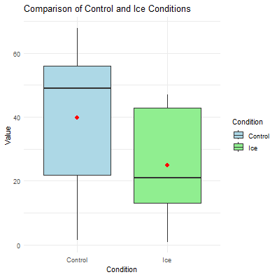
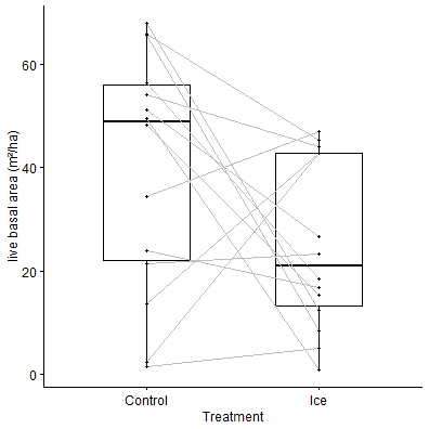
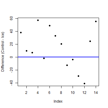
class: center, middle, inverse, title-slide

.title[
# Dependent t-tests
]
.author[
### Pablo E. Gutiérrez-Fonseca
]
.date[
### 2024-10-10
]

---

# Dependent t-test

- Used when we have dependent samples - matched, paired or tied somehow:
  - Repeated measures
  - Brother & sister, husband & wife
  - Left hand, right hand, etc.

- Useful to **control individual differences**.  Can result in more powerful test than independent samples t-test.

---
# Assumptions

1. The dependent variable must be continuous.

2. The two groups are paired.

3. No significant outliers in the difference between the two related groups.

4. The **difference** between the two related treatment groups should be **normally distributed**.

---
# Function

.pull-left[

``` r
t.test(x= , y = ,
       `mu = 0`, 
       paired = , 
       var.equal =, 
       alternative = c("two.sided", "less", "greater")
       )
```
]

.pull-right[

- The `mu` argument indicate the true value of difference in means for a two sample test.

]

---
# Function

.pull-left[

``` r
t.test(x= , y = ,
       `mu = 0`, 
       paired = , 
       var.equal =, 
       alternative = c("two.sided", "less", "greater")
       )
```
]

.pull-right[

- The `mu` argument indicate the true value of difference in means for a two sample test.

- Hypotheses testing for mean difference ( `$\mu_d$` ):

- `$H_0: \mu_d = 0$`

- `$H_1: \mu_d \neq 0$` (two-tailed)
  - `$H_1: \mu_d > 0$` (upper-tailed)
  - `$H_1: \mu_d < 0$` (lower-tailed)

]

---
# Example

- Background About the Experiment:

- During the winters of 2015 and 2016, scientists simulated ice storms in the Hubbard Brook Experimental Forest in New Hampshire by spraying water onto the forest canopy, creating ice accretion that mimicked natural storm conditions. Some plots received ¼ inch, ½ inch, or ¾ inch of ice, while treatments were repeated in 2017 to study the effects of consecutive storms.

- Task:

- Your task is to determine if live basal area (m²/ha) is significantly greater in control plots compared to ice-treated plots, using data collected one year after the initial treatment.

- Additional Information: <a href="https://hubbardbrook.org/story/the-ice-storm-experiment-at-hubbard-brook/">Link </a>

---
# Import your data

``` r
ice_before_after <- read_csv("Lecturer Practice/ice_storm_data_before_and_after.csv") 
head(ice_before_after)
```

```
## # A tibble: 6 × 3
##   Plot_ID Control   Ice
##     <dbl>   <dbl> <dbl>
## 1       1    56.5 18.5 
## 2       2    54.0 44.1 
## 3       3    23.8 16.8 
## 4       4    65.6  8.36
## 5       5    21.3 23.3 
## 6       6    49.5  0.81
```

---
# Run descriptive statistics

``` r
pivot(ice_before_after, c(IQR, skew, kurtosis, mean, sd, var), Ice)
```

```
##   n na    IQR  skew   kurt   mean     sd     var
##  14  0 29.678 0.148 -1.577 24.952 16.484 271.715
```

``` r
pivot(ice_before_after, c(IQR, skew, kurtosis, mean, sd, var), Control)
```

```
##   n na    IQR  skew   kurt   mean     sd     var
##  14  0 33.973 -0.48 -1.196 39.689 23.387 546.956
```

---
#  Test for normality

``` r
shapiro.test(ice_before_after$Control)
```

```
## 
## 	Shapiro-Wilk normality test
## 
## data:  ice_before_after$Control
*## W = 0.90344, p-value = 0.1266
```

``` r
shapiro.test(ice_before_after$Ice)
```

```
## 
## 	Shapiro-Wilk normality test
## 
## data:  ice_before_after$Ice
*## W = 0.89493, p-value = 0.09523
```

---
# Test for equal variance (homogeneity in variances)

``` r
var.test(ice_before_after$Control, ice_before_after$Ice)
```

```
## 
## 	F test to compare two variances
## 
## data:  ice_before_after$Control and ice_before_after$Ice
*## F = 2.013, num df = 13, denom df = 13, p-value = 0.2205
## alternative hypothesis: true ratio of variances is not equal to 1
## 95 percent confidence interval:
##  0.6462141 6.2705042
## sample estimates:
## ratio of variances 
##            2.01298
```

---
# Data visualization

.panelset[
.panel[.panel-name[R Code]

``` r
# Convert data to long format for ggplot
ice_before_after_long <- ice_before_after %>%
  pivot_longer(cols = c("Control", "Ice"), 
               names_to = "Condition", 
               values_to = "Value")
ggplot(ice_before_after_long, aes(x = Condition, y = Value, fill = Condition)) +
  geom_boxplot() +
  stat_summary(fun = mean, geom = "point", shape = 20, size = 4, color = "red", fill = "red") + theme_minimal() +
  labs(title = "Comparison of Control and Ice Conditions",
       x = "Condition", y = "Value") +
  scale_fill_manual(values = c("lightblue", "lightgreen"))
```
]

.panel[.panel-name[Plot]
![](Dependent-t-test_files/figure-html/plot1-1.png)
]
]

---
# Data visualization

.panelset[
.panel[.panel-name[R Code]

# Step 2: Create the paired boxplot with connected points
ggpaired(ice_before_after_long, x = "Condition", y = "Value", 
         id = "ID",                # Using 'ID' to connect paired points
         order = c("Control", "Ice"), 
         line.color = "gray",       # Line color for connections
         line.size = 0.5,           # Line thickness
         boxplot = TRUE) +          # Adding boxplot
  labs(x = "Treatment", y = "live basal area (m²/ha)")
```
]

.panel[.panel-name[Plot]
![](Dependent-t-test_files/figure-html/plot2-1.png)
]
]

---

# Mental check for paired or unpaired

Paired!

<center>
<img src="fig/someone.png" alt="" width="300"/>
  
  
---

#8. Run the code for the appropriate test

``` r
t.test(ice_before_after$Control, ice_before_after$Ice,
alternative = c("greater"),
mu = 0, 
paired = TRUE, 
var.equal = TRUE,
conf.level = 0.95)
```

```
## 
## 	Paired t-test
## 
## data:  ice_before_after$Control and ice_before_after$Ice
*## t = 1.8109, df = 13, p-value = 0.04666
## alternative hypothesis: true mean difference is greater than 0
## 95 percent confidence interval:
##  0.3250056       Inf
## sample estimates:
## mean difference 
##        14.73643
```

---
# Simple plot of differences

- A simple plot of differences between one sample and the other.  Points below the blue line indicate observations where Ice is greater than Control, that is where (Control - Ice) is negative.

.panelset[
.panel[.panel-name[R Code]

``` r
Difference = ice_before_after$Control - ice_before_after$Ice

plot(Difference,
     pch = 16,
     ylab="Difference (Control - Ice)")

abline(0,0, col="blue", lwd=2)
```
]

.panel[.panel-name[Plot]
![](Dependent-t-test_files/figure-html/plot3-1.png)
]
]
---
# Effect size

``` r
effectsize::cohens_d(ice_before_after$Control, ice_before_after$Ice,data=ice_before_after)
```

```
## Cohen's d |        95% CI
## -------------------------
## 0.73      | [-0.04, 1.49]
## 
## - Estimated using pooled SD.
```
---