Factorial ANOVA

class: center, middle, inverse, title-slide

.title[
# Factorial ANOVA
]
.author[
### Pablo E. Gutiérrez-Fonseca
]
.date[
### 2024-10-28
]

---

# What is a Full Factorial Experiment?
- A factorial experiment allows researchers to study the joint **effect of two or more factors** on a **dependent variable**.

- Factorial designs are an **extension of single factor ANOVA** designs in which additional factors are added such that each level of one factor is applied to all levels of the other factor(s) and these combinations are replicated.

---
# Treatment Groups in Full Factorial Design
- Factor A has two levels (i.e., A1 and A2), factor B has three levels (i.e., B1, B2 and B3). Therefore, the full factorial design has 2 x 3 = 6 treatment groups.

|         | B1            | B2            | B3            |
|---------|---------------|---------------|---------------|
| A1      | Group 1      | Group 2      | Group 3      |
| A2      | Group 4      | Group 5      | Group 6      |

---
# Decision Flowchart: Testing Process

<div id="htmlwidget-c4f53a9771377bab9e1b" style="width:900px;height:600px;" class="DiagrammeR html-widget "></div>
<script type="application/json" data-for="htmlwidget-c4f53a9771377bab9e1b">{"x":{"diagram":"\n    graph TD;\n\n        A[What type of data?] --> B[Continuous] \n        A --> Z[Categorical]\n        \n        B --Research Question--> C[Comparing Differences] \n        B --Research Question--> D[Examining Relationships]\n        \n        C --> E[How many groups?] \n      \n        E --1 group--> F[Normally distributed?] \n        F --Yes--> G[One-sample z-test] \n        F --No--> H[Wilcoxon signed rank test]\n        \n        E --2 groups--> I[Are Samples Independent?] \n        I --Yes--> J[Normally distributed?]\n        I --No--> K[Normally distributed?]\n        \n        J --Yes--> L[Independent t-test] \n        J --No--> M[Wilcoxon rank sum test] \n        \n        K --Yes--> N[Paired t-test] \n        K --No--> O[Wilcoxon matched pair test]\n        \n        E --More than 2 groups--> P[Number of Treatments?]\n        \n        P --One--> Q[Normally Distributed?]\n        Q --Yes--> R[One-Way ANOVA]\n        Q --No--> S[Non-Parametric ANOVA]\n        \n        P --More than One--> T[Normally Distributed?]\n        \n        T --Yes--> U[Factorial ANOVA]\n        T --No--> V[Friedman's Rank Test]\n\n  style A fill:lightblue,stroke:#333,stroke-width:1px\n  style B fill:lightblue,stroke:#333,stroke-width:1px\n  style C fill:lightblue,stroke:#333,stroke-width:1px\n  style D fill:lightblue,stroke:#333,stroke-width:1px\n  style E fill:lightblue,stroke:#333,stroke-width:1px\n  style F fill:lightblue,stroke:#333,stroke-width:1px\n  style G fill:lightblue,stroke:#333,stroke-width:1px\n  style H fill:lightblue,stroke:#333,stroke-width:1px\n  style I fill:lightblue,stroke:#333,stroke-width:1px\n  style J fill:lightblue,stroke:#333,stroke-width:1px\n  style K fill:lightblue,stroke:#333,stroke-width:1px\n  style L fill:lightblue,stroke:#333,stroke-width:1px\n  style M fill:lightblue,stroke:#333,stroke-width:1px\n  style N fill:lightblue,stroke:#333,stroke-width:1px\n  style O fill:lightblue,stroke:#333,stroke-width:1px\n  style P fill:lightblue,stroke:#333,stroke-width:1px\n  style Q fill:lightblue,stroke:#333,stroke-width:1px\n  style R fill:lightblue,stroke:#333,stroke-width:1px\n  style S fill:lightblue,stroke:#333,stroke-width:1px\n  style T fill:lightblue,stroke:#333,stroke-width:1px\n  style U fill:lightblue,stroke:#333,stroke-width:1px\n  style V fill:lightblue,stroke:#333,stroke-width:1px\n  style Z fill:lightblue,stroke:#333,stroke-width:1px\n\n  "},"evals":[],"jsHooks":[]}</script>

---
# One-way ANOVA Summary Table

- `$c$` = number of groups.  
- `$n$` = number of observations.

---
# Factorial ANOVA Summary Table

| Source of<br/> Variation          |   Degrees of<br/> Freedom (DF)   |     Sum of Squares<br/> (SS)     |     Mean Square<br/> (MS)   |        F-value        |
|----------------------------------|:----------------------------------:|:----------------------------------:|:---------------------------:|:---------------------:|
| **Factor A**                     |          `$a - 1$`                  |             `$SSA$`                 |    `$MSA = \frac{SSA}{a - 1}$`  |       `$\frac{MSA}{MSW}$`  |
| **Factor B**                     |          `$b - 1$`                  |             `$SSB$`                 |    `$MSB = \frac{SSB}{b - 1}$`  |       `$\frac{MSB}{MSW}$`  |
| **Interaction (A × B)**         |          `$(a - 1)(b - 1)$`         |             `$SS_{AB}$`             |    `$MS_{AB} = \frac{SS_{AB}}{(a - 1)(b - 1)}$` |   `$\frac{MS_{AB}}{MSW}$`  |
| **Within<br/> Groups**           |          `$N - ab$`                 |             `$SSW$`                 |    `$MSW = \frac{SSW}{N - ab}$`  |                       |
| **Total**                        |          `$N - 1$`                  |      `$SST = SSA + SSB + SS_{AB} + SSW$`            |                           |                       |

- `$a$` = number of levels in Factor A.  
- `$b$` = number of levels in Factor B.  
- `$N$` = total number of observations.

---
# When do you do a Factorial ANOVA
- You have a continuous response variable.

- You have two or more categorical treatment variables (factors).

- You want to simultaneously test for differences in the response variable across these factors.

- You want to block for a source of known variability to better isolate the effect of the main variables of interest.

- You suspect there may be interactions between the factors that could influence the response, potentially hiding the true relationships.

---
# ANOVA Terminology

- **One-Way ANOVA**: Used when you have one treatment variable. The non-parametric alternative is the **Kruskal-Wallis test**.

- **Factorial ANOVA**: Applied when there are two or more treatment variables. The name reflects the number of groups and variables, e.g., a 2x3 Factorial ANOVA. The non-parametric alternative is Friedman’s k-way test.

- **Full Factorial ANOVA**: Used when you are also considering interaction terms between variables. This analysis examines the **main effects** and **interactions** among factors.

---
# Factorial ANOVA ANOVA test hypotheses

- Two-way ANOVA Test Hypotheses:

- `$H_{0A}: \mu_{A1} = \mu_{A2} = \dots = \mu_{Ak}$` 
(There is no difference in the means of factor A).

- `$H_{0B}: \mu_{B1} = \mu_{B2} = \dots = \mu_{Bk}$` 
(There is no difference in the means of factor B).

- `$H_{0AB}$`: There is no interaction between factors A and B.

---
# Factorial ANOVA ANOVA test hypotheses

- Two-way ANOVA Test Hypotheses:

- `$H_{0A}: \mu_{A1} = \mu_{A2} = \dots = \mu_{Ak}$` 
(There is no difference in the means of factor A).

- `$H_{0B}: \mu_{B1} = \mu_{B2} = \dots = \mu_{Bk}$` 
(There is no difference in the means of factor B).

- `$H_{0AB}$`: There is no interaction between factors A and B.

- Alternative Hypotheses:

- `$H_{1A}$`: The means for factor A are not equal.

- `$H_{1B}$`: The means for factor B are not equal.

- `$H_{1AB}$`: There is an interaction between factors A and B.

---
# Assumptions of two-way ANOVA test
- Two-way ANOVA, like all ANOVA tests, makes the following assumptions:

- The observations within each cell are normally distributed.
- The variances across groups are equal (homogeneity of variances).

---
# Example

``` r
crop <- read.csv('Lecturer Practice/crop.csv')
head(crop)
```

```
##   density block fertilizer    yield
## 1     low     1       ctrl 177.2287
## 2    high     2       ctrl 177.5500
## 3     low     3       ctrl 176.4085
## 4    high     4       ctrl 177.7036
## 5     low     1       ctrl 177.1255
## 6    high     2       ctrl 176.7783
```

---
# Data visualization
- Visualize the data distribution using boxplots and jitter for individual points:

.panelset[
.panel[.panel-name[R Code]

``` r
ggplot(crop) +
  aes(x = fertilizer, y = yield, fill = density) +
  geom_boxplot(position = position_dodge(width = 0.75), alpha = 0.6, outlier.shape = NA) +
  geom_jitter(aes(color = density), shape = 15, position = position_jitterdodge(jitter.width = 0.2, dodge.width = 0.75)) +
  theme_minimal() +
  labs(title = "Yield by Fertilizer and Density",
       x = "Fertilizer",
       y = "Yield") +
  theme(legend.position = "right") +
  scale_fill_manual(values = c("low" = "lightblue", "high" = "lightcoral")) +
  scale_color_manual(values = c("low" = "blue", "high" = "red"))
```
]

.panel[.panel-name[Plot]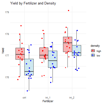
![](Factorial-ANOVA_files/figure-html/plot1-1.png)
]
]

---
# Running the Full Factorial ANOVA
- Run Full Factorial ANOVA to assess differences between fertilizer groups:

``` r
interaction <- aov(yield ~ fertilizer*density, data = crop)

summary(interaction)
```

```
##                    Df Sum Sq Mean Sq F value   Pr(>F)    
*## fertilizer          2  6.068   3.034   9.001 0.000273 ***
*## density             1  5.122   5.122  15.195 0.000186 ***
*## fertilizer:density  2  0.428   0.214   0.635 0.532500    
## Residuals          90 30.337   0.337                     
## ---
## Signif. codes:  0 '***' 0.001 '**' 0.01 '*' 0.05 '.' 0.1 ' ' 1
```

---
# Data visualization
- Visualize the data distribution using boxplots and jitter for individual points:

.panelset[
.panel[.panel-name[R Code]

``` r
ggplot(crop, aes(x = fertilizer, y = yield, color = density, group = density)) +
  geom_point(position = position_jitter(width = 0.1), size = 2) + # jitter for clarity
  geom_line(stat = "summary", fun = mean, size = 1) + # line for mean yield
  stat_summary(fun = mean, geom = "point", size = 3, shape = 18) + # mean points
  labs(title = "Interaction of Fertilizer and Density on Yield",
       x = "Fertilizer Treatment",
       y = "Yield") +
  scale_color_manual(values = c("low" = "blue", "high" = "red"), 
                     labels = c("Low Density", "High Density")) +
  theme_minimal() +
  theme(plot.title = element_text(hjust = 0.5),
        legend.title = element_blank())
```
]

.panel[.panel-name[Plot]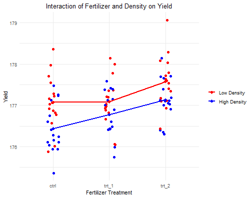
![](Factorial-ANOVA_files/figure-html/plot2-1.png)
]
]

---
# Checking Assumptions: Normality

``` r
# Extract residuals
residuals <- residuals(interaction)
# Perform the Shapiro-Wilk test for normality
shapiro.test(residuals)
```

```
## 
## 	Shapiro-Wilk normality test
## 
## data:  residuals
*## W = 0.98527, p-value = 0.3601
```

---
# Check Assumptions: Homogeneity of Variances
- Perform Levene's Test for homogeneity of variances.

``` r
leveneTest(yield ~ fertilizer * density, data = crop)
```

```
## Levene's Test for Homogeneity of Variance (center = median)
##       Df F value Pr(>F)
*## group  5  0.1589 0.9768
##       90
```

---
# Check Assumptions: Homogeneity of Variances
- Alternatively, use Bartlett's Test if data are normally distributed.

``` r
bartlett.test(yield ~ interaction(fertilizer, density), data = crop)
```

```
## 
## 	Bartlett test of homogeneity of variances
## 
## data:  yield by interaction(fertilizer, density)
*## Bartlett's K-squared = 0.99284, df = 5, p-value = 0.9631
```

---
# Running the Post-hoc Test

``` r
tukey.two.way <- TukeyHSD(interaction)
tukey.two.way
```

```
##   Tukey multiple comparisons of means
##     95% family-wise confidence level
## 
## Fit: aov(formula = yield ~ fertilizer * density, data = crop)
## 
## $fertilizer
##                  diff         lwr       upr     p adj
*## trt_1-ctrl  0.1761687 -0.16972711 0.5220646 0.4482026
*## trt_2-ctrl  0.5991256  0.25322974 0.9450214 0.0002393
*## trt_2-trt_1 0.4229568  0.07706101 0.7688527 0.0123951
## 
## $density
##               diff       lwr        upr     p adj
## low-high -0.461956 -0.697398 -0.2265141 0.0001864
## 
## $`fertilizer:density`
##                              diff         lwr         upr     p adj
## trt_1:high-ctrl:high   0.01364751 -0.58409459  0.61138961 0.9999998
## trt_2:high-ctrl:high   0.50224061 -0.09550149  1.09998271 0.1515870
## ctrl:low-ctrl:high    -0.63489351 -1.23263561 -0.03715141 0.0306553
## trt_1:low-ctrl:high   -0.29620356 -0.89394566  0.30153854 0.7007889
## trt_2:low-ctrl:high    0.06111704 -0.53662506  0.65885914 0.9996758
## trt_2:high-trt_1:high  0.48859310 -0.10914900  1.08633520 0.1742960
## ctrl:low-trt_1:high   -0.64854101 -1.24628311 -0.05079891 0.0254221
## trt_1:low-trt_1:high  -0.30985106 -0.90759316  0.28789104 0.6591096
## trt_2:low-trt_1:high   0.04746953 -0.55027257  0.64521163 0.9999065
## ctrl:low-trt_2:high   -1.13713411 -1.73487621 -0.53939201 0.0000044
## trt_1:low-trt_2:high  -0.79844416 -1.39618626 -0.20070206 0.0025700
## trt_2:low-trt_2:high  -0.44112357 -1.03886567  0.15661853 0.2721714
## trt_1:low-ctrl:low     0.33868995 -0.25905215  0.93643205 0.5680611
## trt_2:low-ctrl:low     0.69601054  0.09826844  1.29375264 0.0128711
## trt_2:low-trt_1:low    0.35732059 -0.24042151  0.95506269 0.5089536
```

---
# Visualizing the Post-hoc Test

- The plot below visualizes the results of the Tukey HSD test:

``` r
tukey.plot.test <- TukeyHSD(interaction)
plot(tukey.plot.test, las = 1)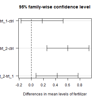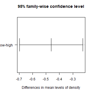
```

![](Factorial-ANOVA_files/figure-html/unnamed-chunk-9-1.png)![](Factorial-ANOVA_files/figure-html/unnamed-chunk-9-2.png)![](Factorial-ANOVA_files/figure-html/unnamed-chunk-9-3.png)

---
# How to summarize results

<span style="color:#00796B;">In this analysis, we examined the effect of fertilizer type and planting density on crop yield</span> <span style="color:#E65100;"> using a two-way ANOVA.</span> 
<span style="color:#1E88E5;"> Results showed that both fertilizer type and planting density significantly influenced yield, with fertilizer having an `$F_{(2, 90)} =9.001, p<0.001 , r^2 =$` and density showing an even stronger effect with `$F_{(1,90)} = 15.195, p<0.001 , r^2 =$`. However, the interaction between fertilizer and density was not significant `$F_{(2,90)} =0.635 , p=0.532 , r^2 =$`, indicating that the effect of fertilizer on yield does not depend on planting density. A post-hoc Tukey’s HSD test revealed specific differences between fertilizer treatments: crops receiving the second fertilizer type showed significantly higher yields than the control group `$(p<0.001)$`, and also had significantly higher yields than the first fertilizer treatment `$(p=0.012)$`. Additionally, crops grown at lower planting densities had significantly higher yields than those grown at higher densities `$(p<0.001)$`. </span><span style="color:#424242;"> These results suggest that choosing an effective fertilizer and managing planting density are crucial for optimizing crop yield. However, the lack of a significant interaction indicates that adjustments in planting density do not change the relative effectiveness of the fertilizers tested.