The leafdecay package is designed to facilitate the analysis of leaf litter decomposition.
Leaf litter decomposition is an ecosystem process widely used to determine the ecological integrity of streams, as it reflects the chemical (e.g., nutrients), physical (e.g., discharge, geomorphology), and biological (e.g., microorganisms) conditions of the streams.
The organic matter breakdown is a source of dissolved and particulate organic carbon, and influences directly and indirectly on the energy source of stream food webs.
Decomposition rates can be affected by mechanical factors, fungal biomass, and macroinvertebrate abundance and richness.
To install the latest developmental version from github you will need the R package devtools (NOT YET IN CRAN):
devtools::install_github("PEGutierrezF/leafdecay")
leafdecay is under development and we welcome comments, suggestions, or feature requests. If you find a bug in the newest version, please email Pablo E. Gutiérrez-Fonseca (pabloe.gutierrezfonseca at gmail.com)
Please cite leafdecay as follows:
Gutiérrez-Fonseca, P.E. & A. M. Alonso-Rodríguez. 2020. leafdecay: a package for leaf litter decomposition analysis in R. R package version 1.0.0.
Classen-Rodríguez, L., Gutiérrez-Fonseca, P.E. & A., Ramírez. 2019. Leaf-litter decomposition and macroinvertebrate assemblages along an urban stream gradient in Puerto Rico. Biotropica, 51, 641-651. PDF
To use the leafdecay package, leaf litter decomposition experiments must be designed with:
- An appropriate number of replicates (three to five). Each replica will be composed of several leaf packs that will be periodically sampled. We recommend that replicas be independent. This will facilitate the calculation of the decomposition rate for each replica and subsequent analyzes (e.g., ANOVAs).
- Consider using extra leaf packs to calculate mass loss due to handling (more details below).
- Leaf packs should be periodically sampled (e.g., day: 1, 3, 7, 14, 21 ...) throughout the study (1-2 months). However, this will depend on the conditions of the stream and the leaf type.
For an appropriate design of a litter decomposition experiment, we strongly recommend:
Benfield, E.F., Fritz, K.M., & S.D., Tiegs. (2017). Leaf-litter breakdown. In G. Lamberti, & F. R. Hauer (Eds.). Methods in stream ecology (3rd ed). pp.71-82. Cambridge, MA: Academic Press.
The package offers functions to:
- Quantify mass loss due to handling.
- Determine the leaf mass remaining.
- Calculate the decomposition rate (-k).
- Calculate the regression fit of leaf mass vs. time.
- Visually explore data using 5 types of graphs.
Install leafdecay package
devtools::install_github("PEGutierrezF/leafdecay")
library(leafdecay)
leafdecay requires 7 input objects:
Day: Time in which a leaf pack is collected.
Treatment: Different groups evaluated.
Replicate: Number of independent samples deployed in different pools.
InitialWt: Initial mass (dry mass) of the leaf packs.
FinalWt: Final mass (dry mass) of the leaf packs.
Frac.InitialWt: Initial mass of a fraction of the leaf pack to be burned (AFDM).
Frac.FinalWt : Final mass of a fraction of the leaf pack that has been burned (AFDM).
The easiest way to get these objects into leafdecay is to create an Excel file or similar, and then copying it across as in the following example:
##    Day Treatment Replicate InitialWt FinalWt InitialFraction FinalFraction
## 1    0   Control         1      5.01    4.99          1.1071        0.3858
## 2    0   Control         1      5.01    4.94          1.1964        0.3504
## 3    0   Control         1      5.01    4.84          1.0647        0.4248
## 4    0   Control         1      5.01    4.82          1.0005        0.3333
## 5    0   Control         1      5.01    4.96          1.0453        0.3417
## 6    0   Control         1      5.00    4.97          1.1212        0.3467
## 7    2        CC         1      5.00    4.65          1.0081        0.3229
## 8    4        CC         1      5.00    4.64          1.0898        0.3489
## 9    8        CC         1      5.00    4.17          1.0956        0.4098
## 10  16        CC         1      5.00    4.00          1.0060        0.3345
## 11  32        CC         1      5.01    4.26          1.0472        0.3921
## 12  44        CC         1      5.00    3.70          1.0143        0.3470
## 13   2        CC         2      5.00    4.63          1.0972        0.3605
## 14   4        CC         2      5.01    4.37          1.0750        0.3181
## 15   8        CC         2      5.00    3.72          1.0420        0.3762
## 16  16        CC         2      5.00    3.99          1.1052        0.3595
## 17  32        CC         2      5.01    3.30          1.0843        0.3908
## 18  44        CC         2      5.00    3.75          1.1112        0.3366
## 19   2        CC         3      5.00    4.67          1.1307        0.3304
## 20   4        CC         3      5.00    4.37          1.0295        0.2948
## 21   8        CC         3      5.00    4.12          1.0876        0.3787
## 22  16        CC         3      5.01    3.64          1.0922        0.3511
## 23  32        CC         3      5.00    3.47          1.0177        0.3385
## 24  44        CC         3      5.00    3.30          1.0061        0.3318
## 25   2       QLC         1      5.01    4.91          1.1301        0.2833
## 26   4       QLC         1      5.00    4.52          1.0000        0.2189
## 27   8       QLC         1      5.01    4.54          1.0449        0.3299
## 28  16       QLC         1      5.00    3.66          1.0420        0.3175
## 29  32       QLC         1      5.00    2.46          1.0661        0.3336
## 30  44       QLC         1      5.01    1.82          1.0840        0.2582
## 31   2       QLC         2      5.00    4.66          1.1228        0.3676
## 32   4       QLC         2      5.01    4.25          1.0606        0.3627
## 33   8       QLC         2      5.00    4.02          1.0922        0.3539
## 34  16       QLC         2      5.00    3.33          1.0006        0.3414
## 35  32       QLC         2      5.00    2.29          1.1265        0.4577
## 36  44       QLC         2      5.00    0.90          0.6735        0.2734
## 37   2       QLC         3      5.01    4.68          1.1719        0.3842
## 38   4       QLC         3      5.00    4.58          1.1156        0.3237
## 39   8       QLC         3      5.01    4.02          1.1061        0.3903
## 40  16       QLC         3      5.00    3.21          1.0003        0.3110
## 41  32       QLC         3      5.01    0.90          1.0300        0.2147
## 42  44       QLC         3      5.01    0.37          0.1770        0.0671
Dried leaves are easily broken in handling. Therefore, extra leaf packs are necessary to account for losses during fashioning, transporting, and placing the packs in the stream. The extra leaf packs will be used to correct by "handling losses", and are often called Control.
To load the data into leafdecay use:
control <- manipulation(data= RioPriedras,
                        InitialWt= InitialWt,
                        FinalWt= FinalWt,
                        Treatment= Control)
control
This means that we lost 1.76334% due to handling.
The AFDM() function convert leaf pack dry mass to AFDM remaining (AFDMrem) as percentage. Also, this function converts the values of AFDMrem to LN (Ln.AFDMrem), which makes it easy to compare the remaining leaf mass against time in the following function (slope.k()).
remaining <- AFDM(data= RioPriedras,
                InitialWt= InitialWt,
                FinalWt= FinalWt,
                Frac.InitialWt= InitialFraction,
                Frac.FinalWt= FinalFraction,
                Treatment= Treatment,
                Day= Day,
                Replicate= Replicate)

remaining
##    grp Day Replicate Treatment   AFDMrem Ln.AFDMrem
## 1    1   0         1        CC 98.236660   4.587379
## 2    1   2         1        CC 94.669342   4.550390
## 3    1   4         1        CC 94.465752   4.548237
## 4    1   8         1        CC 84.897023   4.441439
## 5    1  16         1        CC 81.435993   4.399817
## 6    1  32         1        CC 86.556221   4.460794
## 7    1  44         1        CC 75.328294   4.321856
## 8    2   0         2        CC 98.236660   4.587379
## 9    2   2         2        CC 94.262162   4.546080
## 10   2   4         2        CC 88.791240   4.486288
## 11   2   8         2        CC 75.735474   4.327247
## 12   2  16         2        CC 81.232403   4.397314
## 13   2  32         2        CC 67.050593   4.205447
## 14   2  44         2        CC 76.346244   4.335279
## 15   3   0         3        CC 98.236660   4.587379
## 16   3   2         3        CC 95.076522   4.554682
## 17   3   4         3        CC 88.968823   4.488286
## 18   3   8         3        CC 83.879073   4.429376
## 19   3  16         3        CC 73.958836   4.303509
## 20   3  32         3        CC 70.645724   4.257678
## 21   3  44         3        CC 67.184695   4.207445
## 22   4   0         1       QLC 98.236660   4.587379
## 23   4   2         1       QLC 99.763156   4.602799
## 24   4   4         1       QLC 92.022673   4.522035
## 25   4   8         1       QLC 92.245362   4.524452
## 26   4  16         1       QLC 74.513934   4.310986
## 27   4  32         1       QLC 50.083136   3.913684
## 28   4  44         1       QLC 36.979418   3.610361
## 29   5   0         2       QLC 98.236660   4.587379
## 30   5   2         2       QLC 94.872932   4.552538
## 31   5   4         2       QLC 86.353037   4.458444
## 32   5   8         2       QLC 81.843173   4.404805
## 33   5  16         2       QLC 67.795465   4.216495
## 34   5  32         2       QLC 46.622106   3.842075
## 35   5  44         2       QLC 18.323099   2.908162
## 36   6   0         3       QLC 98.236660   4.587379
## 37   6   2         3       QLC 95.089932   4.554823
## 38   6   4         3       QLC 93.244212   4.535222
## 39   6   8         3       QLC 81.679814   4.402807
## 40   6  16         3       QLC 65.352385   4.179794
## 41   6  32         3       QLC 18.286525   2.906164
## 42   6  44         3       QLC  7.517794   2.017273
The slope.k() function relates the LN.AFDM values against time to obtain the slope that is equal to the decomposition rate (-k). This procedure is run for each replica, which allows subsequent analyzes using the different -k.
slope.k(remaining,Treatment, Replicate, Day, Ln.AFDMrem)
## # A tibble: 12 x 7
##    Treatment Replicate term        estimate std.error statistic  p.value
##    <chr>         <dbl> <chr>          <dbl>     <dbl>     <dbl>    <dbl>
##  1 CC                1 (Intercept)  4.54      0.0302     150.   2.46e-10
##  2 CC                1 Day         -0.00472   0.00139     -3.39 1.94e- 2
##  3 CC                2 (Intercept)  4.50      0.0511      88.1  3.57e- 9
##  4 CC                2 Day         -0.00611   0.00236     -2.59 4.87e- 2
##  5 CC                3 (Intercept)  4.53      0.0306     148.   2.69e-10
##  6 CC                3 Day         -0.00832   0.00141     -5.90 2.00e- 3
##  7 QLC               1 (Intercept)  4.64      0.0236     197.   6.40e-11
##  8 QLC               1 Day         -0.0229    0.00109    -21.1  4.44e- 6
##  9 QLC               2 (Intercept)  4.66      0.0942      49.5  6.39e- 8
## 10 QLC               2 Day         -0.0343    0.00434     -7.91 5.20e- 4
## 11 QLC               3 (Intercept)  4.78      0.106       44.9  1.03e- 7
## 12 QLC               3 Day         -0.0593    0.00490    -12.1  6.81e- 5
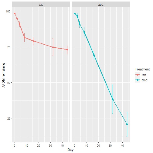
Now, we show 5 plots that can be used to explore your data. However, we strongly suggest improving the plots for publications according to the requirements of journals.
Plot of mean (SD) by treatment.